
From an input
to a useful output.
Three small workflows you can inspect, download and reproduce with the browser tools. Every dataset and part below is synthetic.
These are example workflows, not customer projects or experimental findings. Files open locally in the tools; no account is required.
Make the error bars explicit.
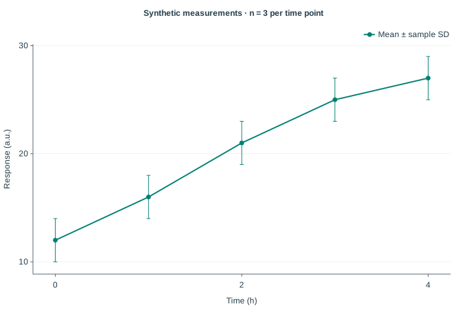
Fifteen synthetic response measurements, three at each of five time points. The figure shows the mean and ±1 sample standard deviation (SD).
Input and method
At 0 h, the values are 10, 12 and 14 a.u.: n = 3, mean = 12 a.u. and sample SD = 2 a.u. Calculate each time point separately, then supply the summary and SD column to Graph Studio.
Mean = Σx / nSample SD = √[Σ(x − mean)² / (n − 1)]
SD describes spread among these observations. It is not SEM, a confidence interval or a measurement uncertainty budget. The connecting line is a visual guide; no regression is fitted.
Reproduce it
- Open Replicate Statistics. Import the 0 h CSV with comma delimiter, a header and column 1; assign the unit
a.u.. The other time points are in the raw table. - Open Graph Studio and choose Open project. Select the downloaded Studio JSON.
- Inspect the summary and raw tables. Panel A maps time to X, mean to Y, sample SD to error bars, and SD as the error meaning. Export SVG to reproduce the output.
Read the browser guide, figure review article and NIST explanation of standard deviation. Need a workflow for your own tables? Explore research workflow services.
Keep dimensions and assumptions together.
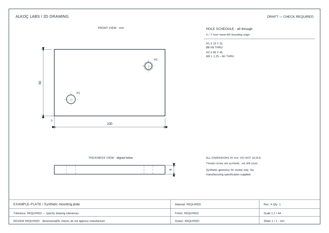
A synthetic 100 × 60 × 8 mm plate with one plain through-hole and one symbolic threaded through-hole.
Input and method
Coordinates start at the lower-left bounding origin, with X right and Y up. H1 is at X = 15, Y = 15, Ø8 H8 through. H2 is at X = 85, Y = 45, M8 × 1.25–6H through.
The drawing tool checks supported geometry, positive edge clearance and non-overlapping holes. Those checks do not establish manufacturing suitability. Thread circles represent nominal diameters, not tap-drill sizes.
Reproduce it
- Download the editable plate JSON and open the Technical Drawing tool.
- Choose Open project, select the JSON and inspect the profile, hole schedule and draft notices.
- Choose Download SVG drawing. For PDF, print A4 landscape at 100% with browser headers and footers disabled.
Single-part review output; not full CAD, GD&T or production release. Read engineering guides and the fits and tolerances article. Explore module adaptation services for a defined drawing workflow.
A cycle you can check by hand.
Synthetic maximum load Fmax = 20 kN and load ratio R = 0.1, with tension positive and compression negative.
Input and method
Use the maximum-plus-ratio definition in the Fatigue & Fracture Workbench. The load-cycle core produces the values shown here; the downloadable note records the same inputs, results and limitations.
- Open the workbench and select Maximum load + load ratio.
- Enter maximum load 20, ratio 0.1 and force unit kN.
- Choose Calculate cycle and compare with the note. Range is twice amplitude.
| Quantity | Definition | Result |
|---|---|---|
| Minimum Fmin | R × Fmax | 2 kN |
| Mean Fmean | (Fmax + Fmin) / 2 | 11 kN |
| Amplitude Fa | (Fmax − Fmin) / 2 | 9 kN |
| Range ΔF | Fmax − Fmin | 18 kN |
These are cycle descriptors, not a fatigue-life or safety prediction. No specimen area, material properties or crack geometry are inferred. R is undefined when Fmax = 0.
Read load-cycle definitions and fatigue input checks. Explore custom calculation and reporting workflows.
One package.
Three worked examples.
Download the common work package, then use Select a work package JSON file in Your Workspace. Inspect the inputs, units, methods and limits before choosing Add reviewed entries. It is a saved record; importing it does not run the tools or replace their editable projects.
Have a related task? Discuss your workflow with its input format, expected output and review requirements.